

 Set up docs MCP
Introduction
This guide focuses on the most common and effective performance optimizations for ClickStack, sufficient to optimize the majority of real-world observability workloads, typically up to tens of terabytes of data per day.
The optimizations are presented in a deliberate order, starting with the simplest and highest impact techniques and progressing toward more advanced and specialized tuning. Early optimizations should be applied first and will often deliver substantial gains on their own. As data volumes grow and workloads become more demanding, the latter techniques become increasingly worthwhile to explore.
ClickHouse concepts
Before applying any of the optimizations described in this guide, it’s important to be familiar with a few core ClickHouse concepts.
In ClickStack, each data source maps directly to one or more ClickHouse tables. When using OpenTelemetry, ClickStack creates and manages a set of default tables that store logs, traces, and metrics data. If you’re using custom schemas or managing your own tables, you may already be familiar with these concepts. However, if you’re simply sending data via the OpenTelemetry Collector, these tables are created automatically, and are where all optimizations described below will be applied.
| Data type | Table |
|---|---|
| Logs | otel_logs |
| Traces | otel_traces |
| Metrics (gauges) | otel_metrics_gauge |
| Metrics (sums) | otel_metrics_sum |
| Metrics (histogram) | otel_metrics_histogram |
| Metrics (Exponential histograms) | otel_metrics_exponentialhistogram |
| Metrics (summary) | otel_metrics_summary |
| Sessions | hyperdx_sessions |
Tables are assigned to databases in ClickHouse. By default, the default database is used - this can be modified in the OpenTelemetry collector.
At a minimum, you should understand the following ClickHouse fundamentals:
| Concept | Description |
|---|---|
| Tables | How data sources in ClickStack correspond to underlying ClickHouse tables. Tables in ClickHouse mainly use the MergeTree engine. |
| Parts | How data is written in immutable parts and merged over time. |
| Partitions | Partitions group the data parts of a table into organised logical units. These units are easier to manage, query, and optimize. |
| Merges | The internal process that merges parts together to ensure that there are a lower number of parts to query. Essential for maintaining query performance. |
| Granules | The smallest unit of data that ClickHouse reads and prunes during query execution. |
| Primary (ordering) keys | How the ORDER BY key determines on-disk data layout, compression, and query pruning. |
These concepts are central to ClickHouse performance. They determine how data is written, how it’s structured on disk, and how efficiently ClickHouse can skip reading data at query time. Every optimization in this guide, whether materialized columns, skip indexes, primary keys, projections, or materialized views, builds on these core mechanisms.
You’re recommended to review the following ClickHouse documentation before undertaking any tuning:
- Creating tables in ClickHouse - A simple introduction to tables.
- Parts
- Partitions
- Merges
- Primary keys/indexes
- How ClickHouse stores data: parts and granules - More advanced guide on how data is structured and queried in ClickHouse, covering granules and primary keys in detail.
- MergeTree- Advanced MergeTree reference guide useful for commands and for internal specifics.
All optimizations described below can be applied directly to the underlying tables using standard ClickHouse SQL, either through the ClickHouse Cloud SQL console or via the ClickHouse client.
Optimization 1. Materialize frequently queried attributes
The first and simplest optimization for ClickStack users is to identify commonly queried attributes in LogAttributes, ScopeAttributes, and ResourceAttributes, and promote them to top-level columns using materialized columns.
This optimization alone is often sufficient to scale ClickStack deployments to tens of terabytes per day and should be applied before considering more advanced tuning techniques.
Why materialize attributes
ClickStack stores metadata such as Kubernetes labels, service metadata, and custom attributes in Map(String, String) columns. While this provides flexibility, querying map subkeys has an important performance implication.
When querying a single key from a Map column, ClickHouse must read the entire map column from disk. If the map contains many keys, this results in unnecessary IO and slower queries compared to reading a dedicated column.
Materializing frequently accessed attributes avoids this overhead by extracting the value at insert time and storing it as a first-class column.
Materialized columns:
- Are computed automatically during inserts
- Can’t be explicitly set in INSERT statements
- Support any ClickHouse expression
- Allow type conversion from String to more efficient numeric or date types
- Enable skip indexes and primary key usage
- Reduce disk reads by avoiding full map access
Example
Consider the default ClickStack schema for traces, where Kubernetes metadata is stored in ResourceAttributes:
CREATE TABLE IF NOT EXISTS ${DATABASE}.otel_traces
(
    `Timestamp` DateTime64(9) CODEC(Delta(8), ZSTD(1)),
    `TraceId` String CODEC(ZSTD(1)),
    `SpanId` String CODEC(ZSTD(1)),
    `ParentSpanId` String CODEC(ZSTD(1)),
    `TraceState` String CODEC(ZSTD(1)),
    `SpanName` LowCardinality(String) CODEC(ZSTD(1)),
    `SpanKind` LowCardinality(String) CODEC(ZSTD(1)),
    `ServiceName` LowCardinality(String) CODEC(ZSTD(1)),
    `ResourceAttributes` Map(LowCardinality(String), String) CODEC(ZSTD(1)),
    `ScopeName` String CODEC(ZSTD(1)),
    `ScopeVersion` String CODEC(ZSTD(1)),
    `SpanAttributes` Map(LowCardinality(String), String) CODEC(ZSTD(1)),
    `Duration` UInt64 CODEC(ZSTD(1)),
    `StatusCode` LowCardinality(String) CODEC(ZSTD(1)),
    `StatusMessage` String CODEC(ZSTD(1)),
    `Events.Timestamp` Array(DateTime64(9)) CODEC(ZSTD(1)),
    `Events.Name` Array(LowCardinality(String)) CODEC(ZSTD(1)),
    `Events.Attributes` Array(Map(LowCardinality(String), String)) CODEC(ZSTD(1)),
    `Links.TraceId` Array(String) CODEC(ZSTD(1)),
    `Links.SpanId` Array(String) CODEC(ZSTD(1)),
    `Links.TraceState` Array(String) CODEC(ZSTD(1)),
    `Links.Attributes` Array(Map(LowCardinality(String), String)) CODEC(ZSTD(1)),
    `__hdx_materialized_rum.sessionId` String MATERIALIZED ResourceAttributes['rum.sessionId'] CODEC(ZSTD(1)),
    `SampleRate` UInt64 MATERIALIZED greatest(toUInt64OrZero(SpanAttributes['SampleRate']), 1) CODEC(T64, ZSTD(1)),
    `ResourceAttributeItems` Array(String) ALIAS arrayMap((arr) -> concat(arr.1, '=', arr.2), ResourceAttributes::Array(Tuple(String, String))),
    `SpanAttributeItems` Array(String) ALIAS arrayMap((arr) -> concat(arr.1, '=', arr.2), SpanAttributes::Array(Tuple(String, String))),
    INDEX idx_trace_id TraceId TYPE bloom_filter(0.001) GRANULARITY 1,
    INDEX idx_rum_session_id __hdx_materialized_rum.sessionId TYPE bloom_filter(0.001) GRANULARITY 1,
    INDEX idx_res_attr_key mapKeys(ResourceAttributes) TYPE bloom_filter(0.01) GRANULARITY 1,
    INDEX idx_res_attr_items ResourceAttributeItems TYPE text(tokenizer = 'array'),
    INDEX idx_span_attr_key mapKeys(SpanAttributes) TYPE bloom_filter(0.01) GRANULARITY 1,
    INDEX idx_span_attr_items SpanAttributeItems TYPE text(tokenizer = 'array'),
    INDEX idx_duration Duration TYPE minmax GRANULARITY 1,
    INDEX idx_lower_span_name lower(SpanName) TYPE tokenbf_v1(32768, 3, 0) GRANULARITY 8
)
ENGINE = MergeTree
PARTITION BY toDate(Timestamp)
ORDER BY (ServiceName, SpanName, toDateTime(Timestamp))
TTL toDate(Timestamp) + ${TABLES_TTL}
SETTINGS index_granularity = 8192, ttl_only_drop_parts = 1;
A user may filter traces using Lucene syntax e.g. ResourceAttributes.k8s.pod.name:"checkout-675775c4cc-f2p9c":
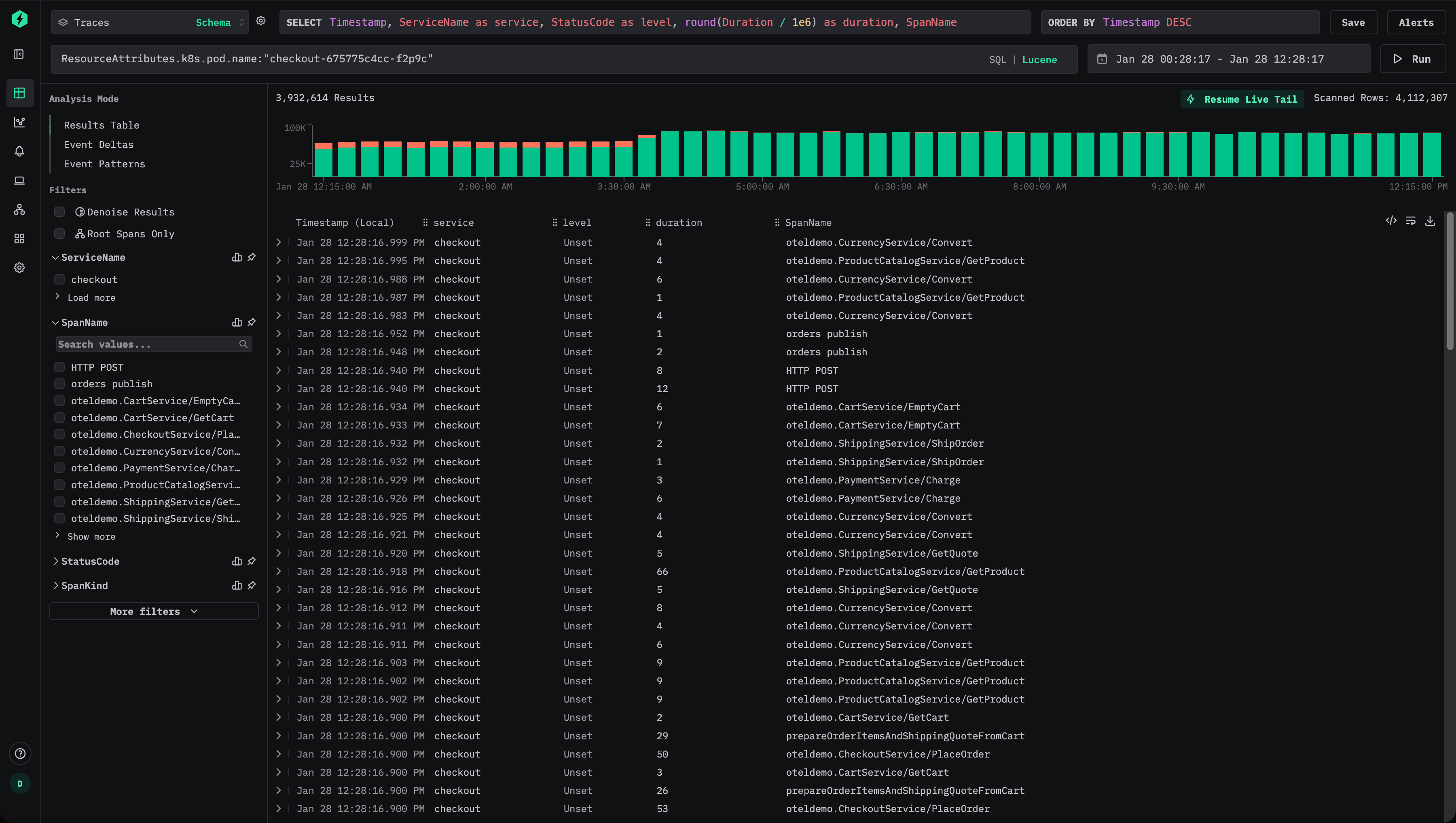
This results in a SQL predicate similar to:
ResourceAttributes['k8s.pod.name'] = 'checkout-675775c4cc-f2p9c'Because this accesses a Map key, ClickHouse must read the full ResourceAttributes column for each matching row - potentially very large if the Map contains many keys.
If this attribute is queried frequently, it should be materialized as a top-level column.
To extract the pod name at insert time, add a materialized column:
ALTER TABLE otel_v2.otel_traces
ADD COLUMN PodName String
MATERIALIZED ResourceAttributes['k8s.pod.name']
From this point forward, new data will store the Pod name as a dedicated column, PodName.
Users can now query for pod names efficiently, using Lucene syntax e.g. PodName:"checkout-675775c4cc-f2p9c"
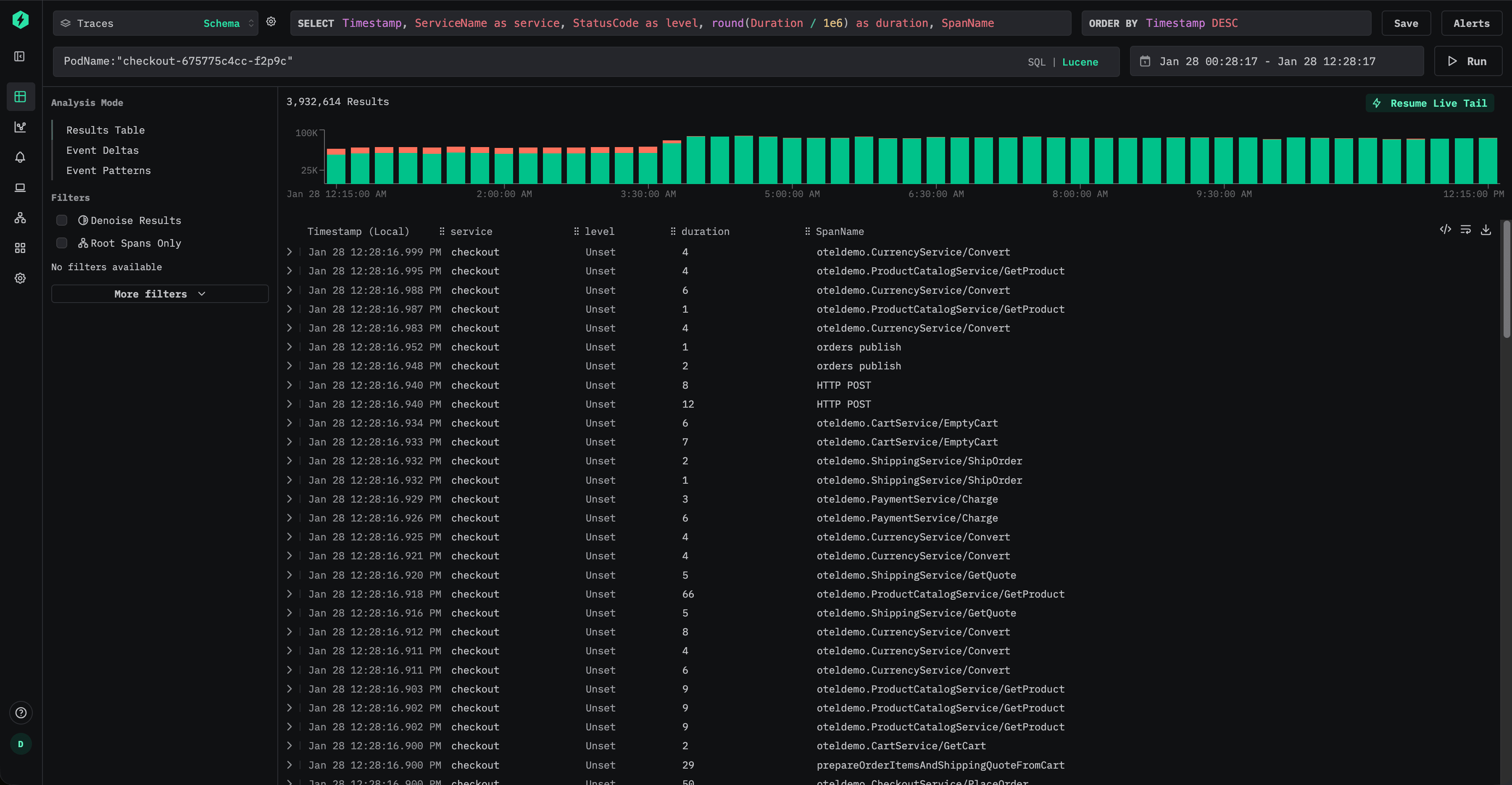
For newly inserted data, this avoids map access entirely and significantly reduces I/O.
However, even if users continue querying the original attribute path e.g. ResourceAttributes.k8s.pod.name:"checkout-675775c4cc-f2p9c", ClickStack will automatically rewrite the query internally to use the materialized PodName column i.e. using the predicate:
PodName = 'checkout-675775c4cc-f2p9c'This ensures users benefit from the optimization without changing dashboards, alerts, or saved queries.
Materializing historical data
Materialized columns only apply automatically to data inserted after the column is created. For existing data, queries against the materialized column will transparently fall back to reading from the original map.
If historical performance is critical, the column can be backfilled using a mutation e.g.
ALTER TABLE otel_v2.otel_traces
MATERIALIZE COLUMN PodName
This rewrites existing parts to populate the column. Mutations are single-threaded per part and can take time on large datasets. To limit impact, mutations can be scoped to a specific partition:
ALTER TABLE otel_v2.otel_traces
MATERIALIZE COLUMN PodName
IN PARTITION '2026-01-02'
Mutation progress can be monitored using the system.mutations table e.g.
SELECT *
FROM system.mutations
WHERE database = 'otel'
  AND table = 'otel_traces'
ORDER BY create_time DESC;
Wait until is_done = 1 for the corresponding mutation.
Optimization 2. Adding skip indexes
After materializing frequently queried attributes, the next optimization is to add data skipping indexes to further reduce the amount of data ClickHouse needs to read during query execution.
Skip indexes allow ClickHouse to avoid scanning entire blocks of data when it can determine that no matching values exist. Unlike traditional secondary indexes, skip indexes operate at the granule level and are most effective when query filters exclude large portions of the dataset. When used correctly, they can significantly accelerate filtering on high-cardinality attributes without changing query semantics.
Consider the default traces schema for ClickStack, which includes skip indexes:
CREATE TABLE IF NOT EXISTS ${DATABASE}.otel_traces
(
    `Timestamp` DateTime64(9) CODEC(Delta(8), ZSTD(1)),
    `TraceId` String CODEC(ZSTD(1)),
    `SpanId` String CODEC(ZSTD(1)),
    `ParentSpanId` String CODEC(ZSTD(1)),
    `TraceState` String CODEC(ZSTD(1)),
    `SpanName` LowCardinality(String) CODEC(ZSTD(1)),
    `SpanKind` LowCardinality(String) CODEC(ZSTD(1)),
    `ServiceName` LowCardinality(String) CODEC(ZSTD(1)),
    `ResourceAttributes` Map(LowCardinality(String), String) CODEC(ZSTD(1)),
    `ScopeName` String CODEC(ZSTD(1)),
    `ScopeVersion` String CODEC(ZSTD(1)),
    `SpanAttributes` Map(LowCardinality(String), String) CODEC(ZSTD(1)),
    `Duration` UInt64 CODEC(ZSTD(1)),
    `StatusCode` LowCardinality(String) CODEC(ZSTD(1)),
    `StatusMessage` String CODEC(ZSTD(1)),
    `Events.Timestamp` Array(DateTime64(9)) CODEC(ZSTD(1)),
    `Events.Name` Array(LowCardinality(String)) CODEC(ZSTD(1)),
    `Events.Attributes` Array(Map(LowCardinality(String), String)) CODEC(ZSTD(1)),
    `Links.TraceId` Array(String) CODEC(ZSTD(1)),
    `Links.SpanId` Array(String) CODEC(ZSTD(1)),
    `Links.TraceState` Array(String) CODEC(ZSTD(1)),
    `Links.Attributes` Array(Map(LowCardinality(String), String)) CODEC(ZSTD(1)),
    `__hdx_materialized_rum.sessionId` String MATERIALIZED ResourceAttributes['rum.sessionId'] CODEC(ZSTD(1)),
    `SampleRate` UInt64 MATERIALIZED greatest(toUInt64OrZero(SpanAttributes['SampleRate']), 1) CODEC(T64, ZSTD(1)),
    `ResourceAttributeItems` Array(String) ALIAS arrayMap((arr) -> concat(arr.1, '=', arr.2), ResourceAttributes::Array(Tuple(String, String))),
    `SpanAttributeItems` Array(String) ALIAS arrayMap((arr) -> concat(arr.1, '=', arr.2), SpanAttributes::Array(Tuple(String, String))),
    INDEX idx_trace_id TraceId TYPE bloom_filter(0.001) GRANULARITY 1,
    INDEX idx_rum_session_id __hdx_materialized_rum.sessionId TYPE bloom_filter(0.001) GRANULARITY 1,
    INDEX idx_res_attr_key mapKeys(ResourceAttributes) TYPE bloom_filter(0.01) GRANULARITY 1,
    INDEX idx_res_attr_items ResourceAttributeItems TYPE text(tokenizer = 'array'),
    INDEX idx_span_attr_key mapKeys(SpanAttributes) TYPE bloom_filter(0.01) GRANULARITY 1,
    INDEX idx_span_attr_items SpanAttributeItems TYPE text(tokenizer = 'array'),
    INDEX idx_duration Duration TYPE minmax GRANULARITY 1,
    INDEX idx_lower_span_name lower(SpanName) TYPE tokenbf_v1(32768, 3, 0) GRANULARITY 8
)
ENGINE = MergeTree
PARTITION BY toDate(Timestamp)
ORDER BY (ServiceName, SpanName, toDateTime(Timestamp))
TTL toDate(Timestamp) + ${TABLES_TTL}
SETTINGS index_granularity = 8192, ttl_only_drop_parts = 1;
These indexes focus on three common patterns:
- High-cardinality string filtering, such as TraceId, session identifiers, attribute keys, or values
- Map subkey filtering accelerated by text indexes on the
*AttributeItemscolumns - Numeric range filtering, such as span duration
The logs table uses text(tokenizer = 'array') indexes throughout instead of Bloom filters, and adds a text(tokenizer = 'splitByNonAlpha') index on lower(Body) for full-text search. See “Tables and schemas used by ClickStack” for the full DDL.
Bloom filters
Bloom filter indexes are the most commonly used skip index type in ClickStack. They’re well-suited for string columns with high cardinality, typically at least tens of thousands of distinct values. A false-positive rate of 0.01 with granularity 1 is a good default starting point and balances storage overhead with effective pruning.
Continuing the example from Optimization 1, suppose the Kubernetes pod name has been materialized from ResourceAttributes:
ALTER TABLE otel_traces
ADD COLUMN PodName String
MATERIALIZED ResourceAttributes['k8s.pod.name']
A Bloom filter skip index can then be added to accelerate filters on this column:
ALTER TABLE otel_traces
ADD INDEX idx_pod_name PodName
TYPE bloom_filter(0.01)
GRANULARITY 1
Once added, the skip index must be materialized - see “Materialize skip index.”
Once created and materialized, ClickHouse can skip entire granules that are guaranteed not to contain the requested pod name, potentially reducing the amount of data read during queries such as PodName:"checkout-675775c4cc-f2p9c".
Bloom filters are most effective when the distribution of values is such that a given value appears in a relatively small number of parts. This often occurs naturally in observability workloads where metadata like pod names, trace IDs, or session identifiers is correlated with time, and therefore clustered by the table’s ordering key.
As with all skip indexes, Bloom filters should be added selectively and validated against real query patterns to ensure they provide measurable benefit - see “Evaluating skip index effectiveness.”
Text indexes
Text indexes offer an alternative to Bloom filters. A Bloom filter is a probabilistic structure that can definitively rule out granules, but it has a false-positive rate, so the granules it doesn’t exclude must still be loaded and evaluated against the WHERE condition. Text indexes are inverted indexes that map tokens to exact offsets within a part. Because they evaluate offsets rather than granules and produce no false positives, they can usually answer the WHERE condition without loading the underlying column. This is an optimization known as direct read. Since loading data is often the largest contributor to query time, direct read can meaningfully reduce query latency.
Additionally, text indexes are themselves queryable, powering autocomplete and other introspection in ClickStack.
Two tokenizers cover most ClickStack patterns:
| Tokenizer | Used for | Typical column |
|---|---|---|
array |
Indexing Array(String) elements as whole tokens |
mapKeys(...), *AttributeItems |
splitByNonAlpha |
Word-level full-text search on prose strings | Body, lower(Body), SpanName |
Array tokenizer for Map and array columns
The default logs schema indexes mapKeys and the materialized item arrays with
the array tokenizer:
INDEX idx_log_attr_key mapKeys(LogAttributes) TYPE text(tokenizer = 'array'),
INDEX idx_log_attr_items LogAttributeItems TYPE text(tokenizer = 'array')
Each Map key (or array element) becomes a single token. Filtering on a known attribute key then prunes any row that does not contain it, without scanning the surrounding Map column. This is the mechanism that makes the Map direct read optimization profitable.
splitByNonAlpha for log bodies
Full-text search on the Body column benefits from a splitByNonAlpha text
index. ClickStack defines this index on lower(Body) so case-insensitive
Lucene searches can use it:
INDEX idx_lower_body lower(Body) TYPE text(tokenizer = 'splitByNonAlpha')When ClickStack detects a text(tokenizer = 'splitByNonAlpha') index on
lower(Body), it rewrites implicit-column Lucene queries like error or
"connection refused" into hasAllTokens(lower(Body), lower(...)), which the
index can satisfy without reading the full Body column. For most
observability log workloads this is the single largest filtering speedup
available.
For a deeper reference on tokenizer options, preprocessors, and verification, see the full-text search documentation.
Text indexes in the default logs schema
The default otel_logs schema synced from upstream ships every text index discussed above: text(tokenizer = 'array') on TraceId, on each mapKeys(...) and *AttributeItems array, and text(tokenizer = 'splitByNonAlpha') on lower(Body) for full-text search. For the canonical DDL, see “Tables and schemas used by ClickStack”; the same schema is reproduced below.
CREATE TABLE IF NOT EXISTS ${DATABASE}.otel_logs
(
  `Timestamp` DateTime64(9) CODEC(Delta(8), ZSTD(1)),
  `TraceId` String CODEC(ZSTD(1)),
  `SpanId` String CODEC(ZSTD(1)),
  `TraceFlags` UInt8,
  `SeverityText` LowCardinality(String) CODEC(ZSTD(1)),
  `SeverityNumber` UInt8,
  `ServiceName` LowCardinality(String) CODEC(ZSTD(1)),
  `Body` String CODEC(ZSTD(1)),
  `ResourceSchemaUrl` LowCardinality(String) CODEC(ZSTD(1)),
  `ResourceAttributes` Map(LowCardinality(String), String) CODEC(ZSTD(1)),
  `ScopeSchemaUrl` LowCardinality(String) CODEC(ZSTD(1)),
  `ScopeName` String CODEC(ZSTD(1)),
  `ScopeVersion` LowCardinality(String) CODEC(ZSTD(1)),
  `ScopeAttributes` Map(LowCardinality(String), String) CODEC(ZSTD(1)),
  `LogAttributes` Map(LowCardinality(String), String) CODEC(ZSTD(1)),
  `EventName` String CODEC(ZSTD(1)),
  `__hdx_materialized_k8s.cluster.name` LowCardinality(String) MATERIALIZED ResourceAttributes['k8s.cluster.name'] CODEC(ZSTD(1)),
  `__hdx_materialized_k8s.container.name` LowCardinality(String) MATERIALIZED ResourceAttributes['k8s.container.name'] CODEC(ZSTD(1)),
  `__hdx_materialized_k8s.deployment.name` LowCardinality(String) MATERIALIZED ResourceAttributes['k8s.deployment.name'] CODEC(ZSTD(1)),
  `__hdx_materialized_k8s.namespace.name` LowCardinality(String) MATERIALIZED ResourceAttributes['k8s.namespace.name'] CODEC(ZSTD(1)),
  `__hdx_materialized_k8s.node.name` LowCardinality(String) MATERIALIZED ResourceAttributes['k8s.node.name'] CODEC(ZSTD(1)),
  `__hdx_materialized_k8s.pod.name` LowCardinality(String) MATERIALIZED ResourceAttributes['k8s.pod.name'] CODEC(ZSTD(1)),
  `__hdx_materialized_k8s.pod.uid` LowCardinality(String) MATERIALIZED ResourceAttributes['k8s.pod.uid'] CODEC(ZSTD(1)),
  `__hdx_materialized_deployment.environment.name` LowCardinality(String) MATERIALIZED ResourceAttributes['deployment.environment.name'] CODEC(ZSTD(1)),
  `ResourceAttributeItems` Array(String) ALIAS arrayMap((arr) -> concat(arr.1, '=', arr.2), ResourceAttributes::Array(Tuple(String, String))),
  `ScopeAttributeItems` Array(String) ALIAS arrayMap((arr) -> concat(arr.1, '=', arr.2), ScopeAttributes::Array(Tuple(String, String))),
  `LogAttributeItems` Array(String) ALIAS arrayMap((arr) -> concat(arr.1, '=', arr.2), LogAttributes::Array(Tuple(String, String))),
  INDEX idx_trace_id TraceId TYPE text(tokenizer = 'array'),
  INDEX idx_res_attr_key mapKeys(ResourceAttributes) TYPE text(tokenizer = 'array'),
  INDEX idx_res_attr_items ResourceAttributeItems TYPE text(tokenizer = 'array'),
  INDEX idx_scope_attr_key mapKeys(ScopeAttributes) TYPE text(tokenizer = 'array'),
  INDEX idx_scope_attr_items ScopeAttributeItems TYPE text(tokenizer = 'array'),
  INDEX idx_log_attr_key mapKeys(LogAttributes) TYPE text(tokenizer = 'array'),
  INDEX idx_log_attr_items LogAttributeItems TYPE text(tokenizer = 'array'),
  INDEX idx_lower_body lower(Body) TYPE text(tokenizer = 'splitByNonAlpha')
)
ENGINE = MergeTree
PARTITION BY toDate(Timestamp)
ORDER BY (toStartOfFiveMinutes(Timestamp), ServiceName, Timestamp)
TTL toDateTime(Timestamp) + ${TABLES_TTL}
SETTINGS index_granularity = 8192, ttl_only_drop_parts = 1, enable_block_number_column = 1, enable_block_offset_column = 1;
Min-max indexes
Minmax indexes store the minimum and maximum value per granule and are extremely lightweight. They’re particularly effective for numeric columns and range queries. While they may not accelerate every query, they’re low-cost and almost always worth adding for numeric fields.
Minmax indexes work best when numeric values are either naturally ordered or confined to narrow ranges within each part.
Suppose a Kafka offset is frequently queried from SpanAttributes:
SpanAttributes['messaging.kafka.offset']This value can be materialized and cast to a numeric type:
ALTER TABLE otel_traces
ADD COLUMN KafkaOffset UInt64
MATERIALIZED toUInt64(SpanAttributes['messaging.kafka.offset'])
A minmax index can then be added:
ALTER TABLE otel_traces
ADD INDEX idx_kafka_offset KafkaOffset TYPE minmax GRANULARITY 1
This allows ClickHouse to efficiently skip parts when filtering by Kafka offset ranges, for example, when debugging consumer lag, or replay behavior.
Again, the index must be materialized prior to it becoming available.
Materialize skip index
After a skip index has been added, it only applies to newly ingested data. Historical data won’t benefit from the index until it’s explicitly materialized.
If you have already added a skip index, for example:
ALTER TABLE otel_traces ADD INDEX idx_kafka_offset KafkaOffset TYPE minmax GRANULARITY 1;You must explicitly build the index for existing data:
ALTER TABLE otel_traces MATERIALIZE INDEX idx_kafka_offset;Materializing a skip index runs as a mutation. Its progress can be monitored using system tables.
SELECT *
FROM system.mutations
WHERE database = 'otel'
  AND table = 'otel_traces'
ORDER BY create_time DESC;
Wait until is_done = 1 for the corresponding mutation.
Once complete, confirm that the index data has been created:
SELECT database, table, name,
       data_compressed_bytes,
       data_uncompressed_bytes,
       marks_bytes
FROM system.data_skipping_indices
WHERE database = 'otel'
  AND table = 'otel_traces'
  AND name = 'idx_kafka_offset';
Non-zero values indicate the index has been successfully materialized.
It’s important the skip index size directly affects query performance. Very large skip indexes, on the order of tens or hundreds of gigabytes, can take noticeable time to evaluate during query execution, which may reduce, or even negate their benefit.
In practice, minmax indexes are typically very small and inexpensive to evaluate, making them almost always safe to materialize. Bloom filter indexes, on the other hand, can grow significantly depending on cardinality, granularity, and false-positive probability.
Bloom filter size can be reduced by increasing the allowed false-positive rate. For example, increasing the probability parameter from 0.01 to 0.05 produces a smaller index that evaluates faster, at the cost of less aggressive pruning. While fewer granules may be skipped, overall query latency can improve due to faster index evaluation.
Tuning Bloom filter parameters is therefore a workload-dependent optimization and should be validated using real query patterns and production-like data volumes.
For further details on skip indexes, see the guide “Understanding ClickHouse data skipping indexes.”
Evaluating skip index effectiveness
The most reliable way to evaluate skip index pruning is to use EXPLAIN indexes = 1, which shows how many parts and granules are eliminated at each stage of query planning. In most cases, you want to see a large reduction in granules at the Skip stage, ideally after the primary key has already reduced the search space. Skip indexes are evaluated after partition pruning and primary key pruning, so their impact is best measured relative to the remaining parts and granules.
EXPLAIN confirms whether pruning occurs, but it doesn’t guarantee a net speedup. Skip indexes have a cost to evaluate, especially if the index is large. Always benchmark queries before and after adding and materializing an index to confirm real performance improvements.
For example, consider the default Bloom filter skip index for TraceId included with the default Traces schema:
INDEX idx_trace_id TraceId TYPE bloom_filter(0.001) GRANULARITY 1You can use EXPLAIN indexes = 1 to see how effective it’s for a selective query:
EXPLAIN indexes = 1
SELECT *
FROM otel_v2.otel_traces
WHERE (ServiceName = 'accounting')
  AND (TraceId = 'aeea7f401feb75fc5af8eb25ebc8e974');

ReadFromMergeTree (otel_v2.otel_traces)
Indexes:
  PrimaryKey
    Keys:
      ServiceName
    Parts: 6/18
    Granules: 255/35898
  Skip
    Name: idx_trace_id
    Description: bloom_filter GRANULARITY 1
    Parts: 1/6
    Granules: 1/255
In this case, the primary key filter reduces the dataset substantially first (from 35898 granules down to 255), and the Bloom filter then prunes that further to a single granule (1/255). This is the ideal pattern for skip indexes: primary key pruning narrows the search, then the skip index removes most of what remains.
To validate the real impact, benchmark the query with stable settings and compare execution time. Use FORMAT Null to avoid result serialization overhead, and disable the query condition cache to keep runs repeatable:
SELECT *
FROM otel_traces
WHERE (ServiceName = 'accountingservice') AND (TraceId = '4512e822ca3c0c68bbf5d4a263f9943d')
SETTINGS use_query_condition_cache = 0
2 rows in set. Elapsed: 0.025 sec. Processed 8.52 thousand rows, 299.78 KB (341.22 thousand rows/s., 12.00 MB/s.)
Peak memory usage: 41.97 MiB.Now run the same query with skip indexes disabled:
SELECT *
FROM otel_traces
WHERE (ServiceName = 'accountingservice') AND (TraceId = '4512e822ca3c0c68bbf5d4a263f9943d')
FORMAT Null
SETTINGS use_query_condition_cache = 0, use_skip_indexes = 0;
0 rows in set. Elapsed: 0.702 sec. Processed 1.62 million rows, 56.62 MB (2.31 million rows/s., 80.71 MB/s.)
Peak memory usage: 198.39 MiB.Disabling use_query_condition_cache ensures results aren’t affected by cached filtering decisions, and setting use_skip_indexes = 0 provides a clean baseline for comparison. If the pruning is effective and index evaluation cost is low, the indexed query should be materially faster, as in the example above.
When to add skip indexes
Skip indexes should be added selectively, based on the types of filters users run most frequently and the shape of the data in parts and granules. The goal is to prune enough granules to offset the cost of evaluating the index itself, which is why benchmarking on production-like data is essential.
For numeric columns that are used in filters, a minmax skip index is almost always a good choice. It’s lightweight, cheap to evaluate, and can be effective for range predicates - especially when values are loosely ordered, or confined to narrow ranges inside parts. Even when minmax doesn’t help a specific query pattern, its overhead is typically low enough that it’s still reasonable to keep.
For string columns, prefer text indexes where supported; fall back to Bloom filters otherwise. Text indexes accelerate the same equality and IN filters that Bloom filters do, and additionally enable token-based predicates (hasToken, hasAllTokens, has) used by full-text search and the Map direct read optimization. On older clusters that don’t yet support text indexes, Bloom filters remain a solid choice.
Bloom filters are most effective for high-cardinality string columns where each value has relatively low frequency, meaning most parts and granules don’t contain the searched value. As a rule of thumb, Bloom filters are most promising when the column has at least 10,000 distinct values, and often perform best with 100,000+ distinct values. They’re also more effective when matching values are clustered into a small number of sequential parts, which typically happens when the column is correlated with the ordering key. Again, your mileage here may vary - nothing replaces real world-testing.
Optimization 3. Map direct read
When you filter on a Map subkey such as LogAttributes['k8s.pod.name'] = 'checkout', ClickHouse must read the entire LogAttributes Map column from
disk and unpack every row to evaluate the predicate. Materializing frequently queried attributes
solves this for keys you know about ahead of time, but it doesn’t scale to
arbitrary attributes that users filter on ad hoc.
Even if a schema has indexes on mapKeys and mapValues, those indexes can tell you whether a row has a given key, and whether it has a given value, but not whether the key and value belong to the same entry. In other words, mapKeys answers mapContainsKey(ResourceAttributes, 'foo') and mapValues answers mapContainsValue(ResourceAttributes, 'bar'), but neither answers ResourceAttributes['foo'] = 'bar'.
By concatenating the keys and values into a single Array(String) column, the
Map direct read optimization enables ResourceAttributes['foo'] = 'bar' to be
answered without loading the underlying map. Maps are often large, and increase
in size with an increase in volume. Combined with an application-level query
rewrite, equality filters on any Map subkey become a single has(...) call
backed by that index, with no Map deserialization at query time. Additionally,
the only storage cost paid is for the text index, as the underlying column is
an ALIAS column and is not stored.
This optimization is automatic. ClickStack ships the necessary columns and indexes in the default logs and trace tables, and rewrites Map subscript filters at runtime when the connected ClickHouse server supports the underlying primitive. If your schema does not contain these columns, or you have additional Map columns you want to accelerate beyond the defaults, read on to enable them.
Schema
For each Map column you want to accelerate, ClickStack defines an
Array(String) ALIAS column that joins each key and value with =:
ALTER TABLE otel_logs
ADD COLUMN LogAttributeItems Array(String)
ALIAS arrayMap(
  (arr) -> concat(arr.1, '=', arr.2),
  LogAttributes::Array(Tuple(String, String))
)
The ALIAS form means the array adds no bytes on disk. ClickHouse computes it at
query time and at index-build time. A text(tokenizer = 'array') skip index on
the ALIAS column stores one token per key=value pair, which ClickHouse uses
to prune granules without touching the source Map:
ALTER TABLE otel_logs
ADD INDEX idx_log_attr_items LogAttributeItems
TYPE text(tokenizer = 'array')
After creating the index on an existing table, materialize it so historical data can use it (see “Materialize skip index”).
The default ClickStack schemas ship these columns and indexes:
| Table | ALIAS columns | Text indexes |
|---|---|---|
otel_logs |
ResourceAttributeItems, ScopeAttributeItems, LogAttributeItems |
idx_res_attr_items, idx_scope_attr_items, idx_log_attr_items |
otel_traces |
ResourceAttributeItems, SpanAttributeItems |
idx_res_attr_items, idx_span_attr_items |
Query rewrite
When a user filters on a Map subkey through the ClickStack UI or the SDK, ClickStack rewrites:
LogAttributes['k8s.pod.name'] = 'checkout'into:
has(LogAttributeItems, concat('k8s.pod.name', '=', 'checkout'))The rewritten form hits the text index on LogAttributeItems, prunes entire
rows that don’t contain the key=value token, and never deserializes the
source LogAttributes Map for non-matching rows. For high-cardinality
observability workloads this typically delivers an order-of-magnitude reduction
in I/O over Map subscript access.
The rewrite happens automatically — saved queries, dashboards, and alerts that
reference LogAttributes['key'] see the speedup without any change.
ClickHouse version requirements
The query rewrite requires a ClickHouse version that supports direct
token-level pruning on text-indexed array columns. ClickStack detects the
connected server version (SELECT version(), cached per connection) and only
emits the rewritten form when the server meets the corresponding threshold
below. Older versions fall back to the original Map subscript form
automatically.
ClickHouse Cloud builds and open-source releases use independent version lines. Use the Cloud minimum versions below.
| ClickHouse branch | Minimum Cloud version |
|---|---|
| 26.2 | 26.2.1.307 |
| 26.3 | 26.3.0.0 |
| 26.4 | 26.4.1.1740 |
| 26.5+ | All versions |
The 26.3.0.0 minimum is the floor of the branch, so all 26.3 builds are
supported.
| ClickHouse branch | Minimum open-source version |
|---|---|
| 26.2 | 26.2.19.43 |
| 26.3 | 26.3.12.3 |
| 26.4 | 26.4.3.37 |
| 26.5+ | All versions |
Optimization 4. Modifying the primary key
The primary key is one of the most important components of ClickHouse performance tuning for most workloads. To tune it effectively, you must understand how it works and how it interacts with your query patterns. Ultimately, the primary key should align with how users access the data, particularly which columns are most commonly filtered on.
While the primary key also influences compression and storage layout, its primary purpose is query performance. In ClickStack, the out-of-the-box primary keys are already optimized for the most common observability access patterns and for strong compression. The default keys for logs, traces, and metrics tables are designed to perform well for typical workflows.
Filtering on columns that appear earlier in the primary key is more efficient than filtering on columns that appear later. While the default configuration is sufficient for most users, there are cases where modifying the primary key can improve performance for specific workloads.
Before modifying any primary key, reading through our guide to understand how primary indexes work in ClickHouse is strongly recommended:
Primary key tuning is table and data-type-specific. A change that benefits one table and data type may not apply to others. The goal is always to optimize for a particular data type e.g. logs.
You will typically optimize the tables for logs and traces. It’s rare that primary key changes need to be made to the other data types.
Below are the default primary keys for the ClickStack tables for logs and traces.
- Logs (
otel_logs) -(toStartOfFiveMinutes(Timestamp), ServiceName, Timestamp) - Traces (
otel_traces) -(ServiceName, SpanName, toDateTime(Timestamp))
See “Tables and schemas used by ClickStack” for the primary keys used by the tables for other data types. Trace tables are optimized for filtering by service name and span name, followed by timestamp. Log tables lead with a five-minute time bucket so time-range scans hit the primary index first, then narrow by service name within each bucket — a layout that suits the common “what happened in the last N minutes for service X” workflow. Although the optimal order is for you to apply filters in the order of the primary key, queries still benefit heavily from filtering on any of these columns in any order, with ClickHouse pruning data prior to reading.
When choosing a primary key, there are also other considerations for choosing an optimal ordering of the columns. See “Choosing a primary key.”
Primary keys should be changed in isolation per table. What makes sense for logs may not make sense for traces or metrics.
Choosing a primary key
First, identify whether your access patterns differ substantially from the defaults for a specific table. For example, if you most commonly filter logs by Kubernetes node before service name, and this represents a dominant workflow, it may justify changing the primary key.
Once you have extracted your desired columns, you can begin optimizing your ordering/primary key.
Some simple rules can be applied to help choose an ordering key. The following can sometimes be in conflict, so consider these in order. Aim to select a maximum of 4-5 keys from this process:
- Select columns that align with your common filters and access patterns. If you typically start Observability investigations by filtering by a specific column e.g. pod name, this column will be used frequently in
WHEREclauses. Prioritize including these in your key over those that are used less frequently. - Prefer columns that help exclude a large percentage of the total rows when filtered, thus reducing the amount of data that needs to be read. Service names and status codes are often good candidates - in the latter case, only if you filter by values which exclude most rows e.g. filtering by 200 codes will, in most systems, match most rows, in comparison to 500 errors, which will correspond to a small subset.
- Prefer columns that are likely to be highly correlated with other columns in the table. This will help ensure these values are also stored contiguously, improving compression.
GROUP BY(aggregations for charts) andORDER BY(sorting) operations for columns in the ordering key can be made more memory efficient.
On identifying the subset of columns for the ordering key, they must be declared in a specific order. This order can significantly influence both the efficiency of the filtering on secondary key columns in queries and the compression ratio for the table’s data files. In general, it’s best to order the keys in ascending order of cardinality. This should be balanced against the fact that filtering on columns that appear later in the ordering key will be less efficient than filtering on those that appear earlier in the tuple. Balance these behaviors and consider your access patterns. Most importantly, test variants. For further understanding of ordering keys and how to optimize them, reading “Choosing a Primary Key.” is recommended for even deeper insights into primary key tuning and the internal data structures, see “A practical introduction to primary indexes in ClickHouse.”
Changing the primary key
If you’re confident of your access patterns prior to data ingestion, simply drop and re-create the table for the relevant data type.
The example below shows a simple way to create a new logs table with the existing schema, but with a new primary key that includes the column SeverityText before the ServiceName.
Create new table
CREATE TABLE otel_logs_temp AS otel_logs
PRIMARY KEY (SeverityText, ServiceName, Timestamp)
ORDER BY (SeverityText, ServiceName, Timestamp)Exchange and drop table
The EXCHANGE statement is used to swap the names of the tables atomically. The temporary table (now the old default table), can be dropped.
EXCHANGE TABLES otel_logs_temp AND otel_logs
DROP TABLE otel_logs_temp
However, the primary key can’t be modified on an existing table. Changing it requires creating a new table.
The following process can be used to ensure the old data can be retained and still queried transparently (using its existing key in the ClickStack UI, if required, while new data is exposed through a new table optimized for the users’ access patterns. This approach ensures ingest pipelines don’t need to be modified, with data still sent to the default table names, and all changes are transparent to users.
The same example of introducing the SeverityText as the first column in the primary key is used below. In this case, a table is created for new data, retaining the old table for historical analysis.
Create new table
Create the new table with the desired primary key. Note the _23_01_2025 suffix - adapt this to be the current date. e.g.
CREATE TABLE otel_logs_23_01_2025 AS otel_logs
PRIMARY KEY (SeverityText, ServiceName, Timestamp)
ORDER BY (SeverityText, ServiceName, Timestamp)
Create a Merge table
The Merge engine (not to be confused with MergeTree) doesn’t store data itself, but allows reading from any number of other tables simultaneously.
CREATE TABLE otel_logs_merge
AS otel_logs
ENGINE = Merge(currentDatabase(), 'otel_logs*')You can now query this table to confirm it returns data from otel_logs.
Update the ClickStack UI to read from the merge table
Configure the ClickStack UI to use otel_logs_merge as the table for the logs data source.
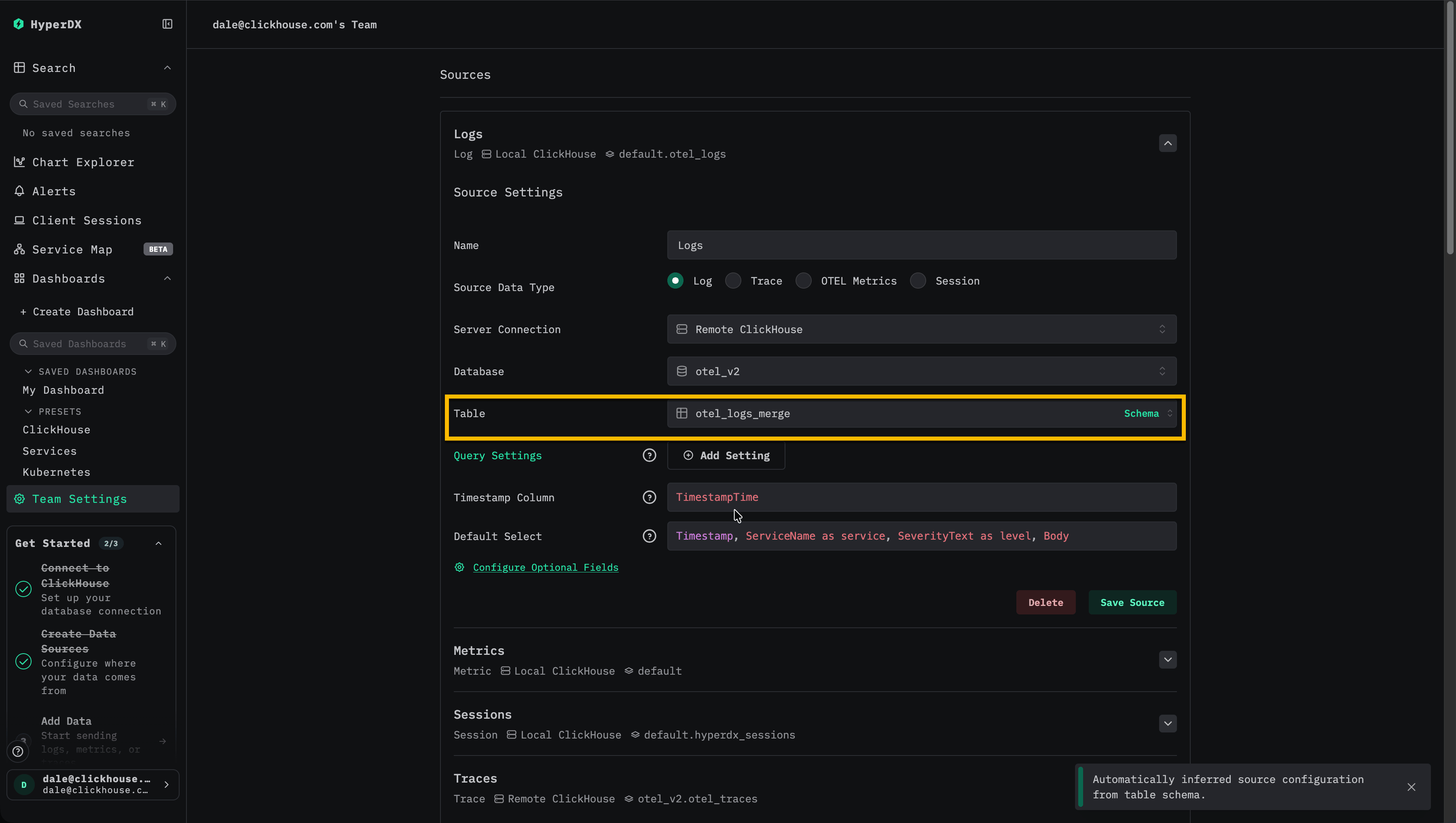
At this point, writes continue to otel_logs with the original primary key, while reads use the merge table. There is no visible change for users or impact on ingestion.
Exchange the tables
An EXCHANGE statement is now used to swap the names of the otel_logs and otel_logs_23_01_2025 tables atomically.
EXCHANGE TABLES otel_logs AND otel_logs_23_01_2025Writes now go to the new otel_logs table with the updated primary key. Existing data remains in otel_logs_23_01_2025 and is still accessible via the merge table. The suffix indicates the date the change was applied and represents the latest timestamp contained in that table.
This process allows primary key changes with no ingest interruption and no user-visible impact.
This process can be adapted should further changes be required to primary keys. For example, if you decide that actually the SeverityNumber should be part of the primary key one week later, rather than the SeverityText. The following process can be adapted as many times as primary key changes are required.
Create new table
Create the new table with the desired primary key.
In the example below 30_01_2025 is used as our suffix to denote the date of the table. e.g.
CREATE TABLE otel_logs_30_01_2025 AS otel_logs
PRIMARY KEY (SeverityNumber, ServiceName, TimestampTime)
ORDER BY (SeverityNumber, ServiceName, TimestampTime)
Exchange the tables
An EXCHANGE statement is now used to swap the names of the otel_logs and otel_logs_30_01_2025 tables atomically.
EXCHANGE TABLES otel_logs AND otel_logs_30_01_2025Writes now go to the new otel_logs table with the updated primary key. The old data remains in otel_logs_30_01_2025, accessible via the merge table.
Row lookup acceleration with block columns
The default ClickStack logs schema enables two MergeTree settings that don’t affect query performance directly, but materially speed up row-detail lookups in the ClickStack UI:
SETTINGS enable_block_number_column = 1, enable_block_offset_column = 1With these settings, every row in the table carries an implicit
(_block_number, _block_offset) pair that uniquely identifies it inside a
part. When you click a log row in the ClickStack UI to open the detail panel, ClickStack
issues a follow-up query to fetch that single row. Without block columns, the
row’s WHERE clause must include enough columns — typically the primary key
plus Body and SeverityText — to disambiguate the row. With block columns,
the primary key plus _block_number plus _block_offset is sufficient. Large
columns like Body are never read for the lookup, effectively speeding up the query.
ClickStack detects the setting from the table’s CREATE statement and emits
the leaner WHERE clause automatically when both columns are enabled. No
application config change is required.
To opt into the optimization on an existing logs or traces table:
ALTER TABLE otel_logs
MODIFY SETTING enable_block_number_column = 1, enable_block_offset_column = 1
The settings apply to data written after the ALTER. Existing parts continue
to use the old per-row lookup until they’re rewritten by a merge.
Optimization 5. Exploiting materialized views
Beta featureClickStack can exploit Incremental Materialized Views to accelerate visualizations that rely on aggregation-heavy queries, such as computing average request duration per minute over time. This feature can dramatically improve query performance and is typically most beneficial for larger deployments, around 10 TB per day and above, while enabling scaling into the petabytes-per-day range. Incremental Materialized Views are in Beta and should be used with care.
For details on using this feature in ClickStack, see our dedicated guide “ClickStack - Materialized Views.”
Optimization 6. Exploiting Projections
Projections represent a final, advanced optimization that can be considered once materialized columns, skip indexes, primary keys, and materialized views have been evaluated. While projections and materialized views may appear similar, in ClickStack, they serve different purposes, and are best used in different scenarios.
Practically, a projection can be thought of as an additional, hidden copy of the table that stores the same rows in a different physical order. This gives the projection its own primary index, distinct from the base table’s ORDER BY key, allowing ClickHouse to prune data more effectively for access patterns that don’t align with the original ordering.
Materialized views can achieve a similar effect by explicitly writing rows into a separate target table with a different ordering key. The key difference is that projections are maintained automatically and transparently by ClickHouse, while materialized views are explicit tables that must be registered and selected intentionally by ClickStack.
When a query targets the base table, ClickHouse evaluates the base layout and any available projections, samples their primary indexes, and selects the layout that can produce the correct result while reading the fewest granules. This decision is made automatically by the query analyzer.
In ClickStack, projections are therefore best suited for pure data reordering, where:
- Access patterns are fundamentally different from the default primary key
- It’s impractical to cover all workflows with a single ordering key
- You want ClickHouse to transparently choose the optimal physical layout
For pre-aggregation and metric acceleration, ClickStack strongly prefers explicit materialized views, which give the application layer full control over view selection and usage.
For additional background, see:
Example projections
Suppose your traces table is optimized for the default ClickStack access pattern:
ORDER BY (ServiceName, SpanName, toDateTime(Timestamp))If you also have a dominant workflow that filters by TraceId (or frequently groups and filters around it), you can add a projection that stores rows sorted by TraceId and time:
ALTER TABLE otel_v2.otel_traces
ADD PROJECTION prj_traceid_time
(
    SELECT *
    ORDER BY (TraceId, toDateTime(Timestamp))
);As with other data layout changes, the projection only affects newly written parts. To build it for existing data, materialize it:
ALTER TABLE otel_v2.otel_traces
MATERIALIZE PROJECTION prj_traceid_time;ClickHouse may choose the projection automatically when it estimates that the projection will scan fewer granules than the base layout. Projections are most reliable when they represent a straightforward reordering of the full row set (SELECT *) and the query filters strongly align with the projection’s ORDER BY.
Queries that filter on TraceId (especially equality) and include a time range would benefit from the above projection. For example:
-- Fetch a specific trace quickly
SELECT *
FROM otel_traces
WHERE TraceId = 'aeea7f401feb75fc5af8eb25ebc8e974'
  AND Timestamp >= now() - INTERVAL 1 DAY
ORDER BY Timestamp;

-- Trace-scoped aggregation
SELECT
  toStartOfMinute(Timestamp) AS t,
  count() AS spans
FROM otel_traces
WHERE TraceId = 'aeea7f401feb75fc5af8eb25ebc8e974'
  AND Timestamp >= now() - INTERVAL 1 DAY
GROUP BY t
ORDER BY t;
Queries that don’t constrain TraceId, or that primarily filter on other dimensions that aren’t leading in the projection’s ordering key, typically won’t benefit (and may read via the base layout instead).
In practice, projections are best suited for workflows where you frequently pivot from a broader search to a trace-centric drill down (for example, fetching all spans for a specific TraceId).
Costs and guidance
- Insert overhead: A
SELECT *projection with a different ordering key is effectively writing the data twice, which increases write I/O and can require additional CPU and disk throughput to sustain ingestion. - Use sparingly: Projections are best reserved for genuinely diverse access patterns where a second physical ordering unlocks meaningful pruning for a large share of queries, for example, two teams querying the same dataset in fundamentally different ways.
- Validate with benchmarks: As with all tuning, compare real query latency and resource usage before and after adding and materializing a projection.
For a deeper background, see:
Lightweight projections with _part_offset
Beta feature
Newer ClickHouse versions also support more lightweight projections that store only the projection sorting key plus a _part_offset pointer into the base table, rather than duplicating full rows. This can greatly reduce storage overhead, and recent improvements enable granule-level pruning, making them behave more like true secondary indexes. See:
Alternatives
If you need multiple ordering keys, projections aren’t the only option. Depending on operational constraints and how you want ClickStack to route queries, consider:
- Configuring your OpenTelemetry collector to write to two tables with different
ORDER BYkeys, and create separate ClickStack sources for each table. - Create a materialized view as a copy pipeline i.e. attach a materialized view to the main table that selects raw rows into a secondary table with a different ordering key (a denormalization or routing pattern). Create a source for this target table. Examples can be found here.